Similarity Measures, Distance Measures and Frequent itemsets

Ranked Retrieval¶

Most users incapable of writing Boolean queries
Boolean queries often result in either too few (=0) or too many (1000s) results.
Rather than a set of documents satisfying a query expression, the system returns an ordering over the top documents in the collection

Scoring as basis for Ranked Retrieval¶

A score measures how well document and query "match"
Jaccard Coefficient
- $jaccard(A,B) = |A ∩ B| / |A ∪ B|$
- A and B don’t have to be the same size.
- Always assigns a number between 0 and 1.
- ISSUES
  - It doesn’t consider term frequency
  - Rare terms in a collection are more informative than frequent terms. Jaccard doesn’t consider this information.
  - We need a more sophisticated way of normalising for length
Bag of Words
- Vector representation doesn’t consider the ordering of words in a document
- John is quicker than Mary and Mary is quicker than John have same vectors
Term Frequency:
- The term frequency $tf_{t,d}$ of term t in document d is defined as the number of times that t occurs in d
- We want to use tf when computing query-document match scores.
- We don't want to use Raw Term Frequency as Relevance does not increase proportionally with term frequency.
Log Frequency Weighting:
- The log frequency weight of term t in d is defined as follows: $tf$-$w_{t,d}$ aka $\(w_{t,d} = 1 + log_{10}\ tf_{t,d}\ \ \ \ \ \ when\ tf_{t,d} > 0 \ \ ; otherwise \ 0$\)
- Score for a document-query pair: sum over terms t in both q and d:$\(score=\ \sum_{t\ ∈\ q\ \cap \ d} (1 \ + \ log_{10}\ tf_{t,d}$\)
- Rare terms are more informative than frequent terms; We want a high weight for rare terms
Inverse Document Frequency
- $df_t$ is the document frequency of t: the number of documents that contain t
- We define the idf (inverse document frequency) of t by $\(idf_t \ = \ log_{10}(N/df_t)$\)
- We use log (N/dft) instead of N/dft to “dampen” the effect of idf.
- idf affects the ranking of documents for queries with at least 2 terms
tf-idf weighting
- product of its tf weight and idf weight$\(w_{t,d} = 1+log(tf_{t,d })\ * \ log_{10}(N/df_t)$\)
- Best known weighting scheme in information retrieval
- Alternative names: tf.idf, tf x idf
- Increases with the number of occurrences within a document
- Increases with the rarity of the term in the collection
- Score for a document given a query:$\(score(q,d)\ = \ \sum_{t\ ∈\ q\ \cap \ d}tf.idf_{t,d}$\)

Queries as Vectors¶

Key idea 1: Do the same for queries: represent them as vectors in the space
Key idea 2: Rank documents according to their proximity to the query in this space
proximity = similarity of vectors or proximity ≈ inverse of distance
The reason we do this is to get away from the 'Feast or Famine' condition of Boolean model
Instead: rank more relevant documents higher than less relevant documents
Euclidean Distance
- bad idea -> it is large for vectors of different lengths
- The Euclidean distance between q and d2 is large even though the distribution of terms in the query q and the distribution of terms in the document d2 are very similar.
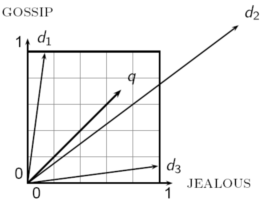
From angles to Cosines
- Ranking documents in decreasing order of the angle between query and document is similar to ranking documents in increasing order of cosine(query, document)
- Cosine is a monotonically decreasing function for the interval [0$\degree$ to 180$\degree$]
- Length Normalization
  - $||\vec{x}|| = \sqrt{\sum_i{x_i^2}}$
  - Dividing a vector by its L2 norm (above formula) makes it a unit (length) vector.
- cosine(query,document)
  - $q_i$ -> tf-idf weight of term i in the query
  - $d_i$ is tf-idf weight of term i in the document $\(cos(\vec{q},\vec{d})\ = \ \frac{\sum_{i=1}^{|V|}q_id_i}{\sqrt{\sum_{i=1}^{|V|}q_i^2}\ \sqrt{\sum_{i=1}^{|V|}d_i^2}}$\)
  - For length-normalized vectors, cosine similarity is simply the dot product $$cos(\vec{q},\vec{d}) = \sum_{i=1}^{|V|}q_id_i $$for q, d length-normalized.
  - calculating Length Normalized Values for a document $\(lengthNormalisedValue_i = \frac{x_i}{\sqrt{x_0^2 + x_1^2.....+x_n^2 }}$\)
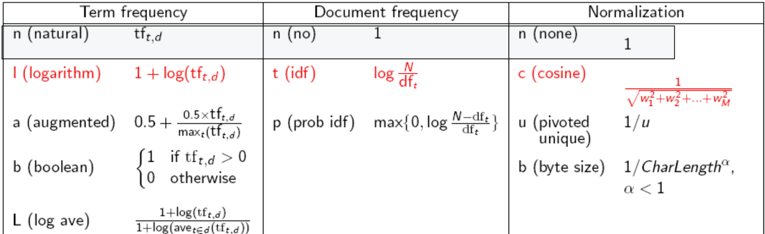
TF-IDF weighting Variants

Similarity Measuring Techniques¶

Shingles
- k-shingle is defined to be any substring of length k found within the document.
- Assumption -> Documents that have lots of shingles in common have similar text, even if the text appears in different order
- You must pick k large enough, or most documents will have most shingles
- Generally value for k used irl is 7-10
Min-Hashing
- Convert large sets to short signatures, while preserving similarity
- Many similarity problems can be formalized as finding subsets that have significant intersection
- $d(C_1,C_2) = 1 - (Jaccard\ Similarity)$
- Representing Sets as Boolean Matrices
  - Rows -> elements (shingles)
  - Columns -> sets(documents)
- Matrix Representation of Set
  - A value 1 in row r and column c if the element for row r is a member of the set for column c
  - Otherwise the value in position (r, c) is 0.
- Hashing Columns (Signatures)
  - Key idea -> “hash” each column C to a small signature h(C), such that:
    - (1) h(C) is small enough that the signature fits in RAM
    - (2) sim(C1, C2) is the same as the “similarity” of signatures h(C1) and h(C2)
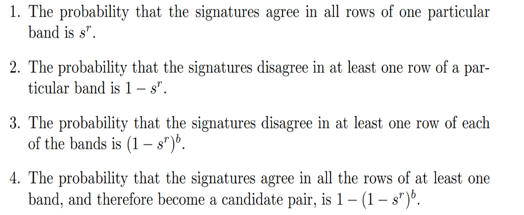
  - Hash docs into buckets. Expect that “most” pairs of near duplicate docs hash into the same bucket!
  - if sim(d1,d2) is high, then the P(H(d1) == H(d2)) is "high"else vice versa
- Permutation
  - Given the following 3 permutations and input matrix; you have to form the signature matrix
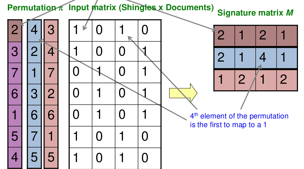
  - the resultant signature matrix will always be in the form (no of permutations X no of documents (columns))
  - fill in column by column i.e.
    - find the first occurrence of 1-valued-bit in increasing order of values of the permutation ; repeat for each permutation
    - For example, in the above row we find:
      - first permutation; (number:value) 1:0, 2:1, 3:1.... we select 2 as it is the lowest occurring valid bit
      - second permutation: 1:0, 2:1... we choose 2
      - third permutation: 1 :1 ... we choose 1
    - repeat above for all documents
- Locality Sensitive Hashing
  - One general approach to LSH is to “hash” items several times, in such a way that similar items are more likely to be hashed to the same bucket than dissimilar items are
  - Any pair that hashed to the same bucket for any of the hashings is termed to be a candidate pair
  - Candidate pairs are the ones that hash to the same bucket
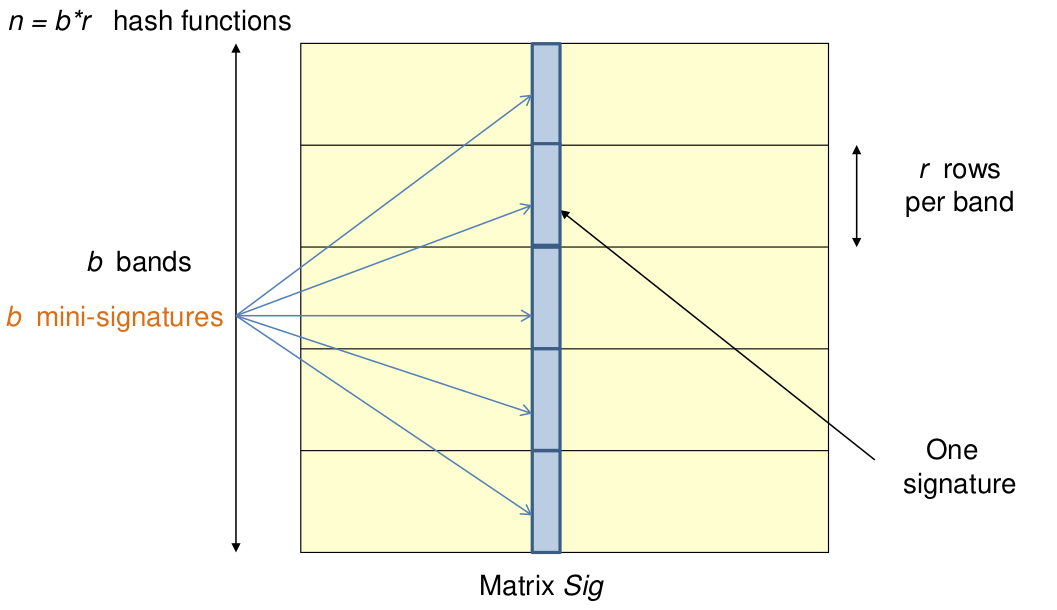
  - • Divide the signature matrix Sig into b bands of r rows
  - • Each band is a mini-signature with r hash functions.

Minimum Edit Room¶

Minimum number of editing operations needed to transform one string into the other
1. Insertion
2. Deletion
3. Substitution
Dynamic Programming solution, tabulation.

Frequent Itemset¶

Itemset with count > minimum support count
Support count ($\sigma$) = Frequency of an itemset
Support -> Fraction of transactions that contain the itemset
Association Rule
- Implication expression of the form X -> Y
  - X and Y are itemsets.
Rule Evaluation Metrics
- Support(s)$\(Support = \frac{\sigma(itemset)}{Total \ Number\ of \ Items}$\)
- Confidence(c)
  - Measures how often item Y appears in transactions that contain X$\(Confidence(c)\ = \frac{X \cap Y}{X}$\)
  - Example, {Milk , Diaper } -> {Beer}$\(Confidence = \frac{\sigma(Milk,Diaper,Beer)}{\sigma(Milk,Diaper)}$\)

Approaches¶

Bruteforce -> Computationally Prohibitive
- Total number of possible association rules: $3^d - 2^{d+1} + 1$
Two-step approach
- Frequent item-set generation
  - Generate all itemsets whose support > minsup
  - Given d items, there are $2^d$ possible candidate itemsets
- Rule Generation
  - Generate high confidence rules from each frequent itemset, where each rule is a binary partitioning of a frequent itemset
Brute-force approach:
- Each itemset in the lattice is a candidate frequent itemset
- Count the support of each candidate by scanning the database
- Complexity O(NMW), Expensive! Since, $M = 2^d$
- Match every transaction against every other
What can be done here then?
- Reduce the number of candidates (M) -> pruning techniques to be used
- Reduce the number of transactions(N) -> reduce size of N as itemset increases
- Reduce the number of comparisons (NM) -> Don't match every candidate with every transaction
Apriori Principle
- If an itemset is frequent, then all of its subsets must also be frequent
- (anti-monotone property) Support of an itemset never exceeds the support of its subsets
Apriori Algorithm:
- Fk: frequent k-itemsets
- Lk: candidate k-itemsets
- Candidate Generation
  1. Bruteforce -> 1 itemset with 1 itemset
  2. Merge $F_{k-1}$ and $F_1$ itemsets
  3. $F_{k-1}$ x $F_{k-1}$ Method
    - Merge two frequent (k-1)-itemsets if their first (k-2) items are identical
    - Alternative method Merge two frequent (k-1)-itemsets if the last (k-2) items of the first one is identical to the first (k-2) items of the second.
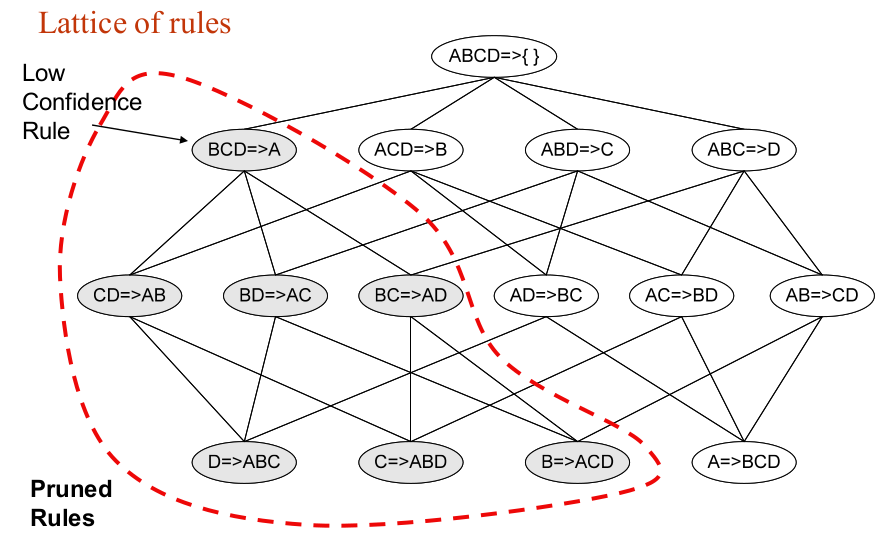
Rule Generation
- Merge two frequent (k-1)-itemsets if the last (k-2) items of the first one is identical to the first (k-2) items of the second.
- But confidence of rules generated from the same itemset has an anti-monotone property$\(c(ABC -> D) ≥ c(AB -> CD) ≥ c(A -> BCD)$\)
Factors Affecting Complexity of Apriori
- Choice of minimum support threshold
  - lowering support threshold results in more frequent itemsets
  - this may increase number of candidates and max length of Frequent itemsets
- Dimensionality (number of items) of the data set
  - More space is needed to store support count of itemsets
  - if number of frequent itemsets also increases, both computation and I/O costs may also increase
- Size of database
  - Run time of algo increases with DB Size
- Average transaction width
  - transaction width increases the max length of frequent itemsets

Maximal Frequent Itemset
- An itemset is maximal frequent if it is frequent and none of its immediate supersets is frequent - In short 'bhai frequent hai, but bhai ki next generation se nahi ho paya!'
Closed Itemset
- An itemset X is closed if none of its immediate supersets has the same support as the itemset X. - ' In short, beta baap se niche hi rahega, equal hua to nahi chalega' - Relationship between the various frequent itemsets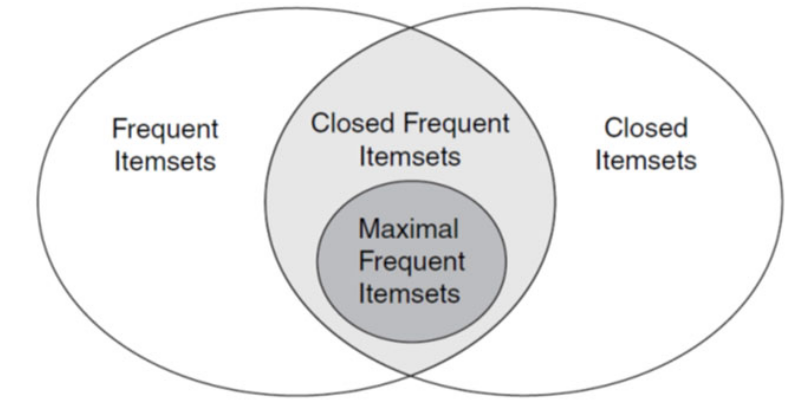 Pasted image 20240501202540.png

- Pattern Evaluation
- Association rule algorithms can produce large number of rules - Interestingness measures can be used to prune/rank the patterns - what kind of rules do we really want?
- Confidence(X -> Y) should be sufficiently high too ensure that people who buy X will more likely buy Y than not buy Y - Confidence(X -> Y) > support(Y) - Otherwise, rule will be misleading because having item X actually reduces the chance of having item Y in the same not buy Yin the same transaction!

Statistical Relationship between X and Y
- If P(X,Y) > P(X) * P(Y) : X & Y are positively correlated - If P(X,Y) < P(X) * P(Y) : X & Y are negatively correlated - P(X,Y) = P(X) * P(Y) (X and Y are independent)

Lift
- Used for rules $\(Lift = \frac{P(Y|X)}{P(Y)}$\)
Interest
- used for itemsets$\(\frac{P(X,Y)}{P(X)P(Y)}$\)
$\(PS = P(X,Y) - P(X)P(Y)$\)

Effect of Support Distribution
- If minsup is too high, we could miss itemsets involving interesting rare items - If minsup is too low, it is computationally expensive and the number of itemsets is very large

A measure of Cross Support
- With n items, we can define a measure of cross support, r as
$\(r(x) = \frac{min{s(x_1),s(x_2),..s(x_n)}}{max{s(x_1),s(x_2),..s(x_n)}}$\) - Can use $r(x)$ to prune cross support patterns - To avoid patterns whose items have very different support, define a new evaluation measure for itemsets